Governing Equations:

Analytical procedure for obtaining limiting active and passive earth pressures - Annex C

(1) The following procedure, which includes certain approximations, may be used in all cases.

(2) The procedure is stated for passive pressures with the strength parameters (represented in the following by ϕ, c, δ, a) inserted as positive values, see Figure C.3.

(3) For active pressures the same algorithm is used, with the following changes:
— the strength parameters ϕ, c, δ and a are inserted as negative values;
— the value of the angle of incidence of the equivalent surface load β0 is β, mainly because of the approximations used for K_γ.

(4) Refer to BS EN 1997-1:2004 Annex C for definitions of symbols used.

(5) The interface parameters δ and a must be chosen so that:

$$ \frac{a}{c} = \frac{\tan\delta}{\tan\varphi} $$

(6) The boundary condition at the soil surface involves β_o, which is the angle of incidence of an equivalent surface load. With this concept the angle is defined from the vectorial sum of two terms:

- actual distributed surface loading q, per unit of surface area, uniform but not necessarily vertical, and;

- c cotϕ acting as normal load.

The angle β_o is positive when the tangential component of q points toward the wall while the normal component is directed toward the soil. If c = 0 while the surface load is vertical or zero, and for active pressures generally, β_o = β.

(7) The angle m_t is determined by the boundary condition at the soil surface:

$$ \cos\left(2m_t + \varphi + \beta_0\right) = -\frac{\sin\beta_0}{\sin\varphi} $$

(8) The boundary condition at the wall determines m_w by:

$$ \cos\left(2m_w + \varphi + \delta\right) = \frac{\sin\delta}{\sin\varphi} $$

The angle m_w is negative for passive pressures (ϕ > 0) if the ratio sin δ /sin ϕ is sufficiently large.

(9) The total tangent rotation along the exterior slip line of the moving soil mass, is determined by the angle v to be computed by the expression

$$ \nu = m_t + \beta - m_w - \theta $$

(10) The coefficient K_n for normal loading on the surface (i.e. the normal earth pressure on the wall from a unit pressure normal to the surface) is then determined by the following expression in which v is to be inserted in radians:

$$ K_n = \frac{1 + \sin\varphi \sin\left(2m_w + \varphi\right)}{1 - \sin\varphi \sin\left(2m_t + \varphi\right)} \exp\left(2\nu \tan\varphi\right) $$

(11) The coefficient for a vertical loading on the surface (force per unit of horizontal area projection), is:

$$ K_q = K_n \cos^2 \beta $$

and the coefficient for the cohesion term is:

$$ K_c = \left(K_n - 1\right) \cot\varphi $$

(12) For the soil weight an approximate expression is:

$$ K_\gamma = K_n \cos\beta \cos\left(\beta - \theta\right) $$

This expression is on the safe side. While the error is unimportant for active pressures it may be considerable for passive pressures with positive values of β.

For ϕ = 0 the following limit values are found:

$$ \begin{align*} \cos 2m_t &= -\frac{p}{c} \sin\beta \cos\beta \,; \\ \cos 2m_w &= \frac{a}{c} \,; \\ K_q &= \cos^2 \beta \,; \\ K_c &= 2\nu + \sin 2m_t + \sin 2m_w \,; \end{align*} $$

(with ν in radians), while for K_γsub> (ϕ = 0), a better approximation is:

$$ K_\gamma = \cos\theta + \frac{\sin\beta \cos m_w}{\sin m_t} $$

(13) Both for passive and active pressures, the procedure assumes the angle of convexity to be positive (ν ≥ 0).

(14) If this condition is not (even approximately) fulfilled, e.g. for a smooth wall and a sufficiently sloping soil surface when β and φ have opposite signs, it may be necessary to consider using other methods. This may also be the case when irregular surface loads are considered.

Important notes extracted from NA.3.2 Annex C

The values of K_a and K_p given in Figures C.1.1 to C.1.4 and Figures C.2.1 to C.2.4 relate to vertical retained faces. Where the retained face is inclined, Equations (C.6) and (C.9) should be used. The note under Equation (C.9) says the expression is on the safe side; this can be taken to mean that it over-estimates the active pressure and under-estimates the passive pressure. When active pressure is favourable and passive pressure is unfavourable the results are therefore not on the safe side.

The values of K_a and K_p given in Figures C.1.1 to C.1.4 and Figures C.2.1 to C.2.4 are based on different theories from those on which Equations C.6 and C.9 are based. The two methods will therefore yield different results when δ is not equal to zero. The equations are more soundly based in theory but there is long experience of use of the graphs. They differ mainly for high values of φ and δ/φ for which it might be difficult to establish the reliability of the experience.

Useful charts from CIRIA C760

Instead of Figures C.1.1 to C.1.4 and Figures C.2.1 to C.2.4 in EC7, Figures A4.15 to A4.23 are reproduced based on the equations given in Annex C of EC7 and presented below.

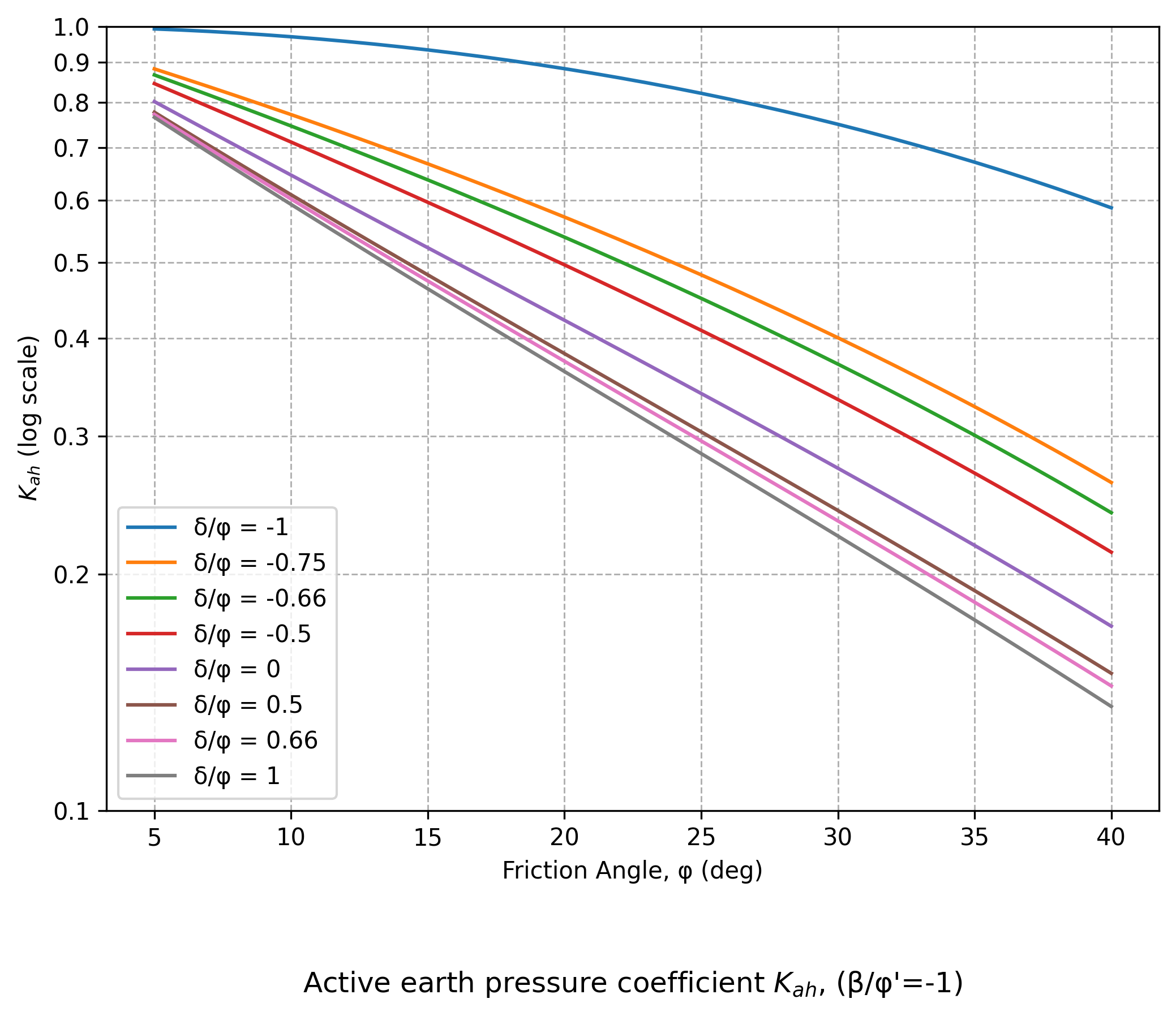
Figure A4.15

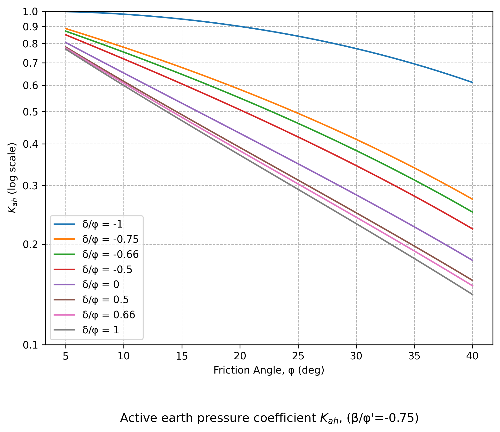
Figure A4.16

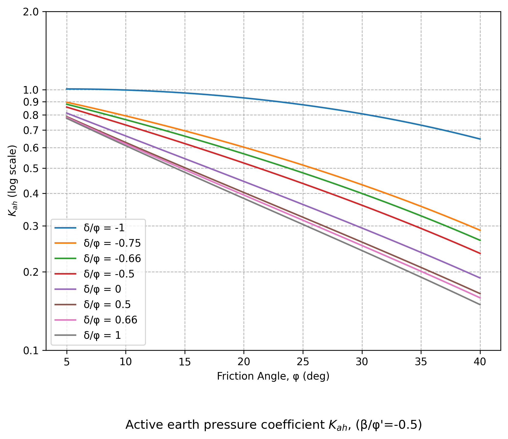
Figure A4.17

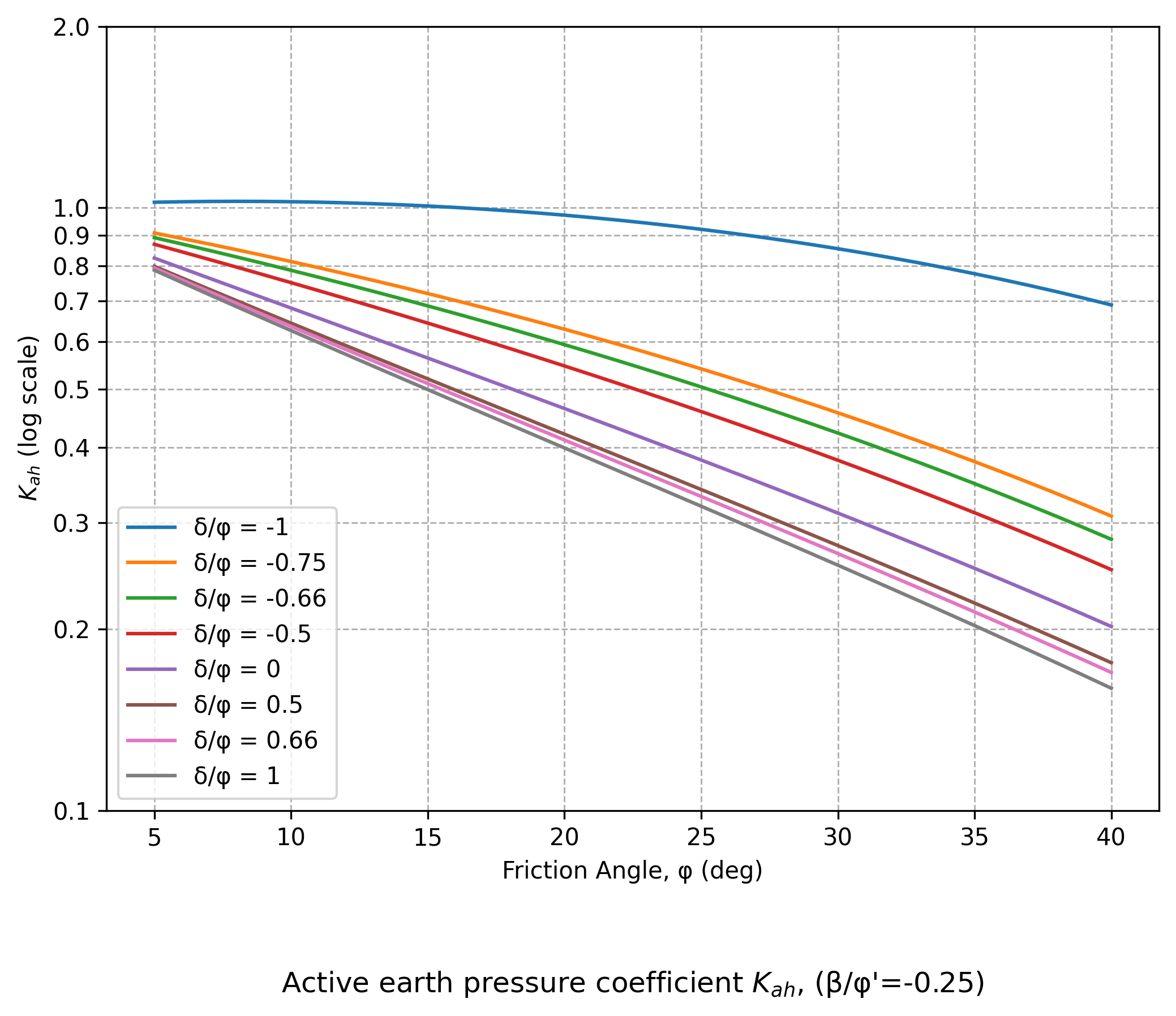
Figure A4.18

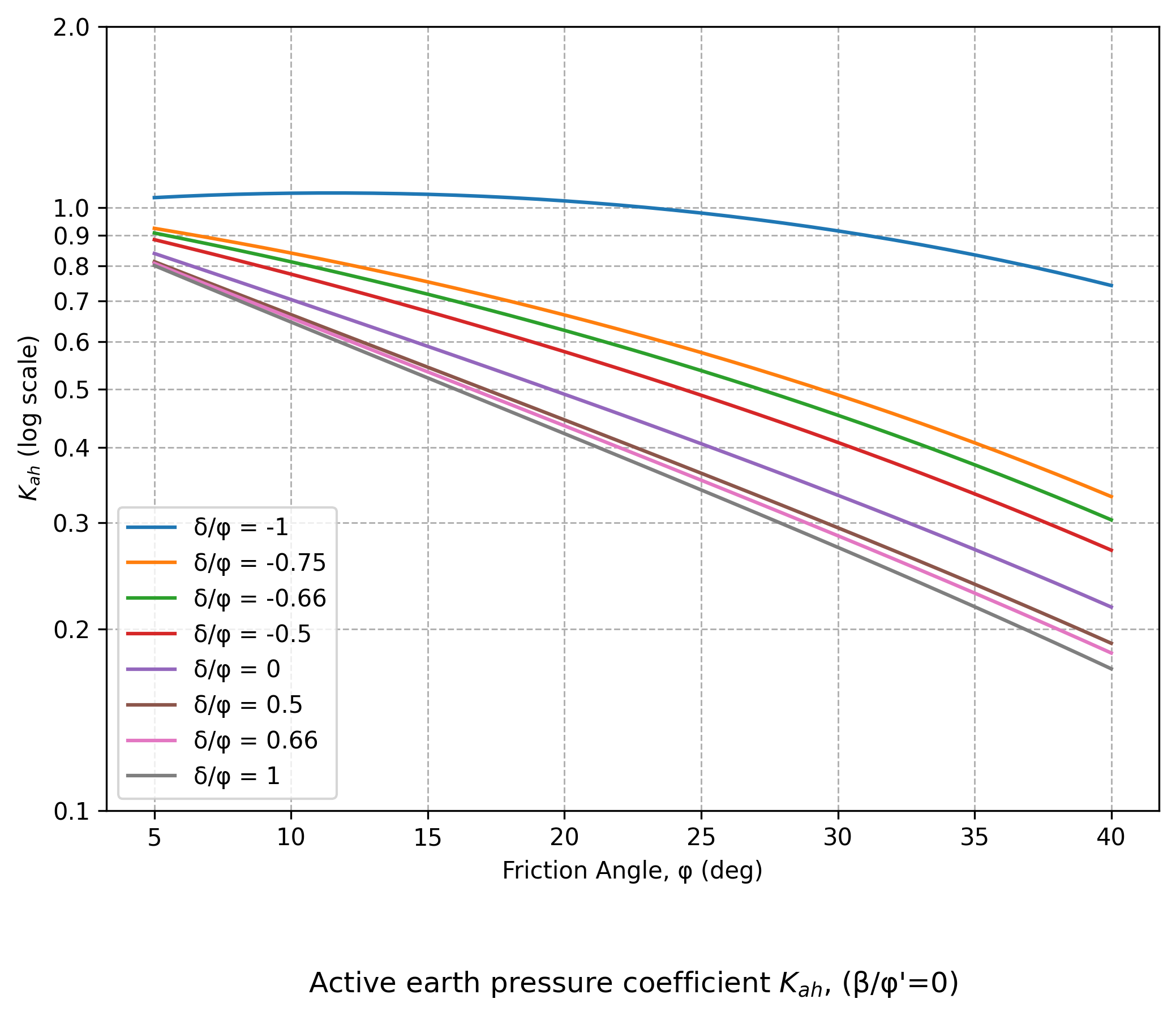
Figure A4.19

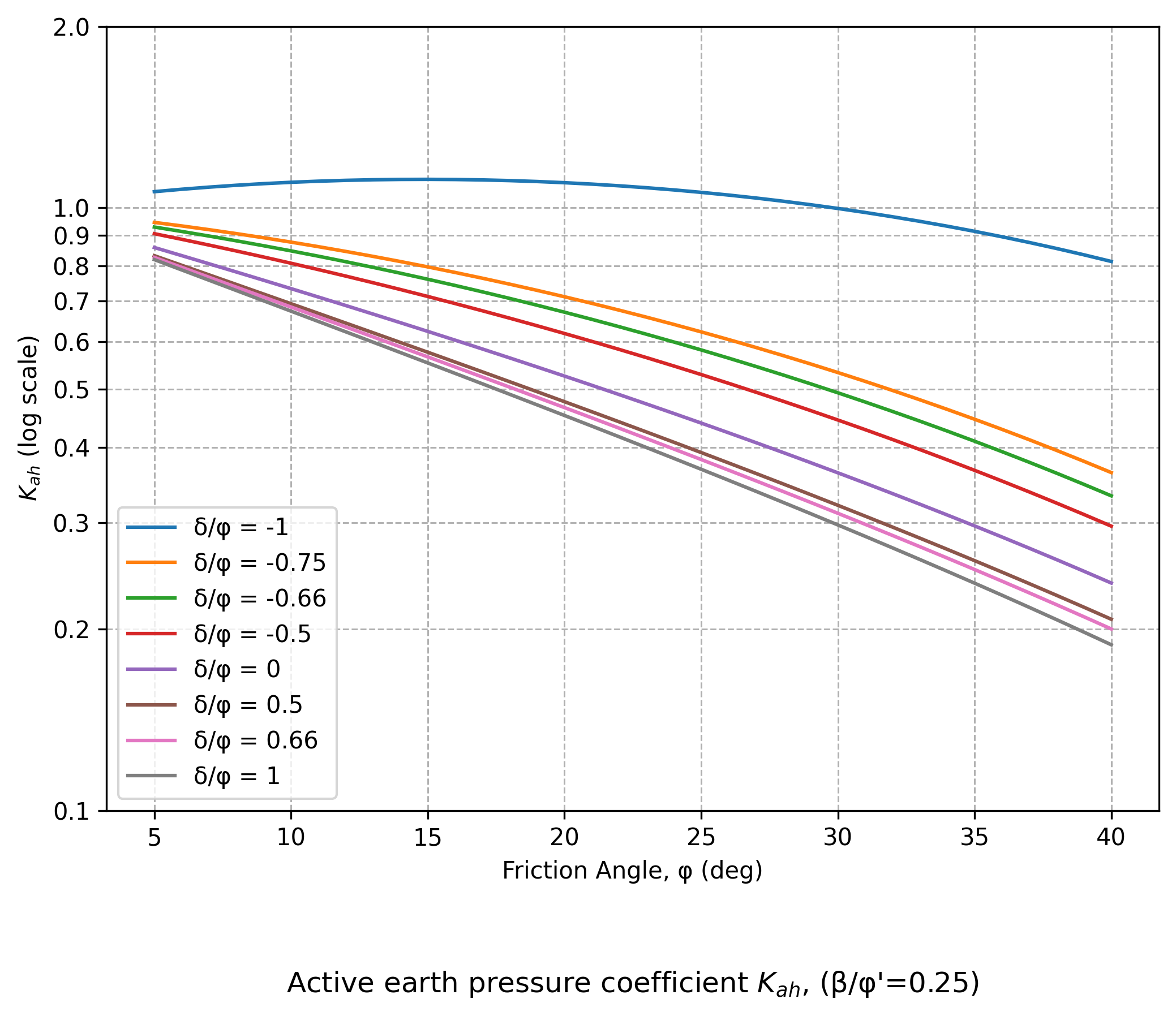
Figure A4.20

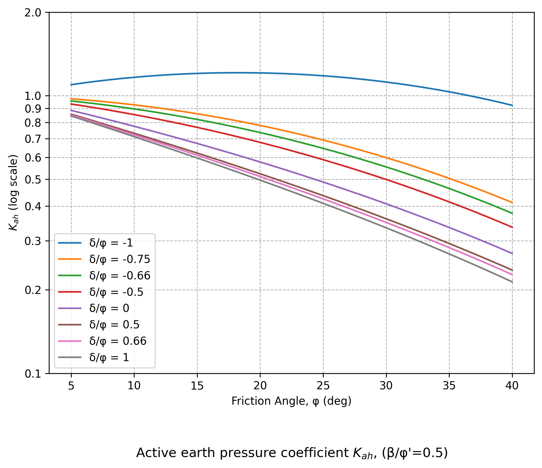
Figure A4.21

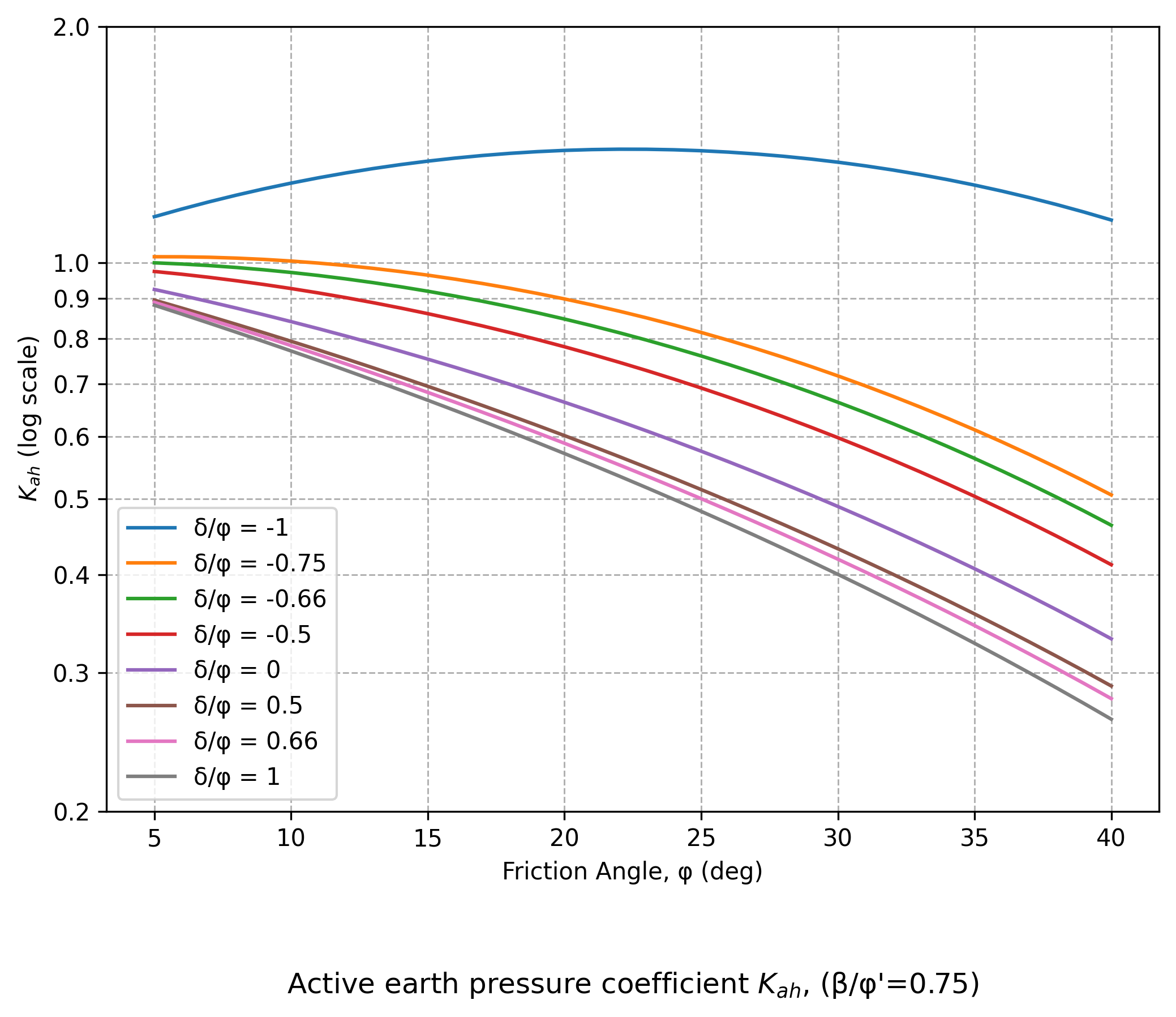
Figure A4.22

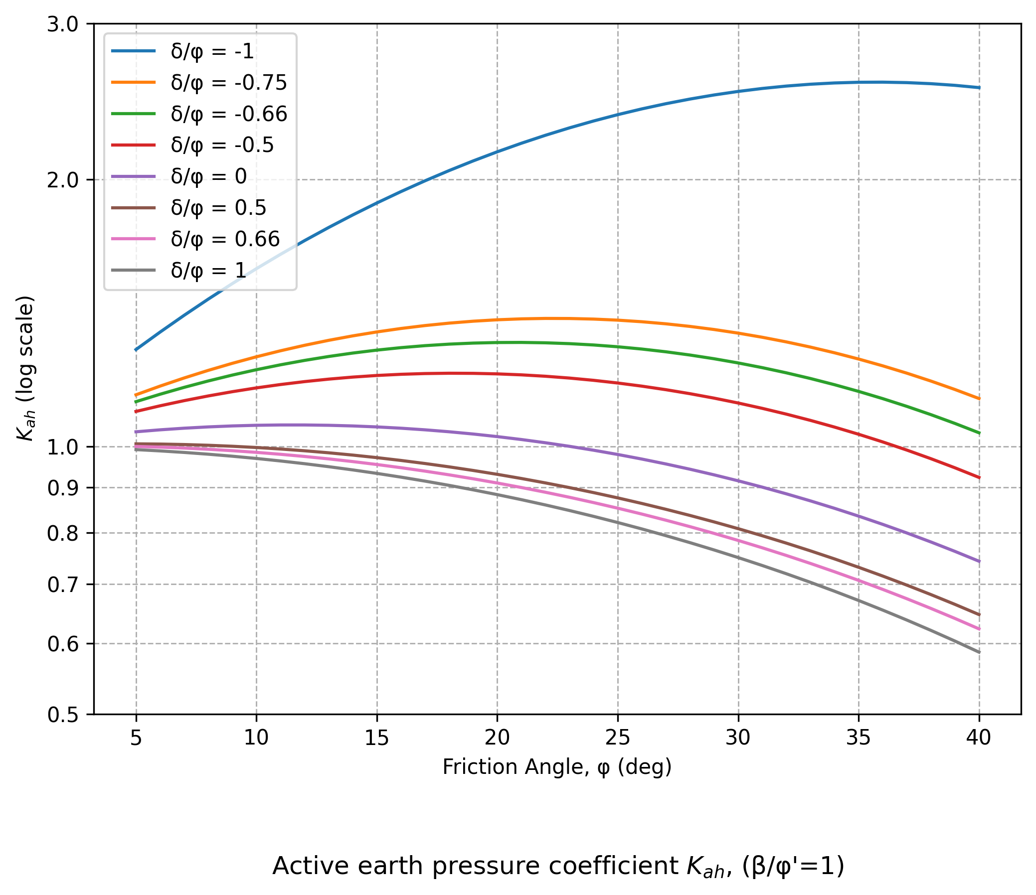
Figure A4.23